Method Tests

Here we discuss all the involved tests, their metrics, thresholds, and the motivation behind the tests.

Introduction

We follow Zhang et al. [ZHML19] and group our tests under the three categories correctness, fairness, robustness. The correctness tests try to make sure that the predictions of the model on the input signal follow the truth as closely as possible for different metrics. The fairness test looks into sub-groups of the data like sex or accent and ensures that the model behaves similar for all sub-groups. The robustness tests investigate how much the model output is affected by changes to input signal like low pass filter or changes in gain.

Random Model

To provide some reference values for the test results we add a random model. For categorical emotion, the random-categorical model randomly samples from a uniform categorical distribution to generate the prediction. For dimensional emotion, the random-gaussian model randomly samples from a truncated Gaussian distribution with values between \(0\) and \(1\), a mean value of \(0.5\), and a standard deviation of \(\frac{1}{6}\).

Fairness Thresholds

For all fairness tests, we use simulations based on random models as reference for setting test thresholds, since a random model has no bias towards certain groups. We simulate the tests by running a random model on random predictions 1000 times under different conditions (number of samples per fairness group, number of fairness groups). The maximum value that occurs in the set of metric results is then used as reference for the respective threshold.

For regression tasks we use the distribution of the random-gaussian model to simulate the predictions as well as the ground truth. For categories, we use the distribution of the (uniform) random-categorical model to simulate the predictions. For the simulation of categorical ground truth, we simulate both a uniform distribution as well as a sparse distribution with the class probabilities \((0.05, 0.05, 0.3, 0.6)\), and select the distribution that applies to the respective test.

For certain test sets, the distribution of the ground truth for certain groups varies from the distribution of other groups. The maximum difference in prediction in the simulation increases under such biases. Therefore we balance the test sets with ground truth labels by selecting 1000 samples from the group with the fewest samples, and 1000 samples from each other group with similar truth samples. For certain regression test sets this results in certain regression bins having very few samples, no longer matching the assumed Gaussian distribution. In these cases, for fairness metrics that involve bins, we skip bins with too few samples. We set the minimum number of samples \(n_{\text{bin}}\) to the expected number of samples in the first bin for a Gaussian distribution with a mean of \(0.5\) and a standard deviation of \(\frac{1}{6}\):

\(n_{\text{bin}} = \mathbb{P}(X\leq0.25) \cdot n\),

where \(n\) is the total number of samples, and the random variable \(X\) follows the aforementioned distribution.

We take the same approach for the tests with unlabelled test sets in the case that a model has very few predictions in a certain bin for the combined test set.

Correctness Classification

The correctness classification tests include standard metrics that are used to evaluate classification problems, namely Precision Per Class, Recall Per Class, Unweighted Average Precision, Unweighted Average Recall.

Overview of tests and thresholds for emotion

Test	Threshold
Precision Per Class	0.5
Recall Per Class	0.5
Unweighted Average Precision	0.5
Unweighted Average Recall	0.5

Correctness Consistency

The correctness consistency tests check whether the models’ predictions on other tasks are consistent with the expected result. For example, we know from the literature that happiness is characterized by high valence and that fear tends to coincide with low dominance [FSRE07]. Based on comparing various literature results [FSRE07, GFSS16, HSS+12, VT17], we expect the following dimensional values for emotional categories:

Emotion categories and their dimensional ranges

	valence	arousal	dominance
anger	low	high	high
boredom	neutral	low
disgust	low
fear	low	high	low
frustration	low
happiness	high		neutral
neutral	neutral	neutral	neutral
sadness	low	low	low
surprise		high	neutral

The Samples in Expected High Range test checks whether the proportion of samples which are expected to have a high value and have a prediction >=0.55 is above a given threshold.

The Samples in Expected Low Range test checks whether the proportion of samples which are expected to have a low value and have a prediction <= 0.45 is above a given threshold.

The Samples in Expected Neutral Range test checks whether the proportion of samples which are expected to have a neutral value and have a prediction in the range of 0.3 and 0.6 is above a given threshold.

Overview of tests and thresholds for arousal

Test	Threshold
Samples In Expected High Range	0.75
Samples In Expected Low Range	0.75
Samples In Expected Neutral Range	0.75

Overview of tests and thresholds for dominance

Test	Threshold
Samples In Expected High Range	0.75
Samples In Expected Low Range	0.75
Samples In Expected Neutral Range	0.75

Overview of tests and thresholds for valence

Test	Threshold
Samples In Expected High Range	0.75
Samples In Expected Low Range	0.75
Samples In Expected Neutral Range	0.75

Correctness Distribution

The distributions as returned from the model for the different test sets should be very similar to the gold standard distributions.

The Jensen Shannon Distance (compare Jensen-Shannon divergence) provides a single value to judge the distance between two random distributions. The value ranges from 0 to 1, with lower values indicating a more similar distribution. We bin the distributions into 10 bins before calculating the distance.

The test Relative Difference Per Class checks that the number of samples per class is comparable between the model prediction and the gold standard. We measure the difference of the number of samples in relative terms compared to the overall number of samples in the test set.

Overview of tests and thresholds for arousal

Test	Threshold
Jensen Shannon Distance	0.2

Overview of tests and thresholds for dominance

Test	Threshold
Jensen Shannon Distance	0.2

Overview of tests and thresholds for valence

Test	Threshold
Jensen Shannon Distance	0.2

Overview of tests and thresholds for emotion

Test	Threshold
Relative Difference Per Class	0.15

Correctness Regression

The correctness regression tests include standard metrics that are used to evaluate regression problems, namely Concordance Correlation Coeff, Pearson Correlation Coeff, Mean Absolute Error.

Overview of tests and thresholds for arousal

Test	Threshold
Concordance Correlation Coeff	0.5
Mean Absolute Error	0.1
Pearson Correlation Coeff	0.5

Overview of tests and thresholds for dominance

Test	Threshold
Concordance Correlation Coeff	0.5
Mean Absolute Error	0.1
Pearson Correlation Coeff	0.5

Overview of tests and thresholds for valence

Test	Threshold
Concordance Correlation Coeff	0.5
Mean Absolute Error	0.1
Pearson Correlation Coeff	0.5

Correctness Speaker Average

The models should be able to estimate the correct average value per speaker. For the classification task, the class proportions should be estimated correctly for each speaker.

We only consider speakers with at least 10 samples for regression, and with at least 8 samples per class for classification.

The test Mean Absolute Error measures the absolute error per speaker.

For the classification task, the test Class Proportion Mean Absolute Error measures the absolute error in the predicted proportion of each class per speaker.

Overview of tests and thresholds for arousal

Test	Threshold
Mean Absolute Error	0.1

Overview of tests and thresholds for dominance

Test	Threshold
Mean Absolute Error	0.1

Overview of tests and thresholds for valence

Test	Threshold
Mean Absolute Error	0.1

Overview of tests and thresholds for emotion

Test	Threshold
Class Proportion Mean Absolute Error	0.1

Correctness Speaker Ranking

For some applications, it may be of interest to create a ranking of speakers in order to spot outliers on either side of the ranking.

The test uses the raw values per sample to calculate the average value for each speaker for regression. For classification, the test uses the proportions per class for each speaker.

We only consider speakers with at least 10 samples for regression, and with at least 8 samples per class for classification.

For the Correctness Speaker Ranking part, keep in mind that these are relative scores and do not represent the absolute accuracy of the prediction. That is why we have the Correctness Speaker Average part.

As a measure of the overall ranking we use Spearman’s rank correlation coefficient (Spearmans Rho), which ranges from 0 to 1.

Overview of tests and thresholds for arousal

Test	Threshold
Spearmans Rho	0.7

Overview of tests and thresholds for dominance

Test	Threshold
Spearmans Rho	0.7

Overview of tests and thresholds for valence

Test	Threshold
Spearmans Rho	0.7

Overview of tests and thresholds for emotion

Test	Threshold
Spearmans Rho	0.7

Fairness Accent

The models should not show a bias regarding the accent of a speaker. For now, we only investigate English accents.

The investigation is based on the speech-accent-archive database, which provides recordings for several different accents. Each speaker in the database was asked to read the same English paragraph, lasting a little longer than 3 minutes in most cases. The database also includes speakers with English as their native language. For each of the 31 accents, there are at least 60 audio samples.

To test the different accents predictions for recordings from speakers with different native languages were collected and compared to the combined database. The accent was named after their native language. For each accent we use recordings from 5 female and 5 male speakers.

The Mean Value over all samples should not change for any specific accent compared to the combined database.

For the test Relative Difference Per Bin we follow Agarwal et al. [ADudikW19] and discretize the regression model outputs into 4 bins. The test checks that the number of samples per bin is comparable between the model prediction for one accent and the model prediction for the combined database. We measure the difference of the number of samples in relative terms compared to the overall number of samples in the test set.

The test Relative Difference Per Class checks that the number of samples per class is comparable between the model prediction for one accent and the model prediction for the combined database. We measure the difference of the number of samples in relative terms compared to the overall number of samples in the test set.

We base the thresholds on simulations with a random-categorical and a random-gaussian model for 30 fairness groups and 60 samples per group. For the test Relative Difference Per Bin we require at least 4 predictions per bin in the combined dataset, or we skip that bin.

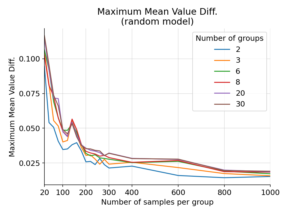
The maximum difference in mean value for a random gaussian model from 1000 simulations.

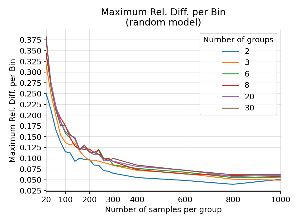
The maximum difference in relative difference per bin for a random gaussian model from 1000 simulations.

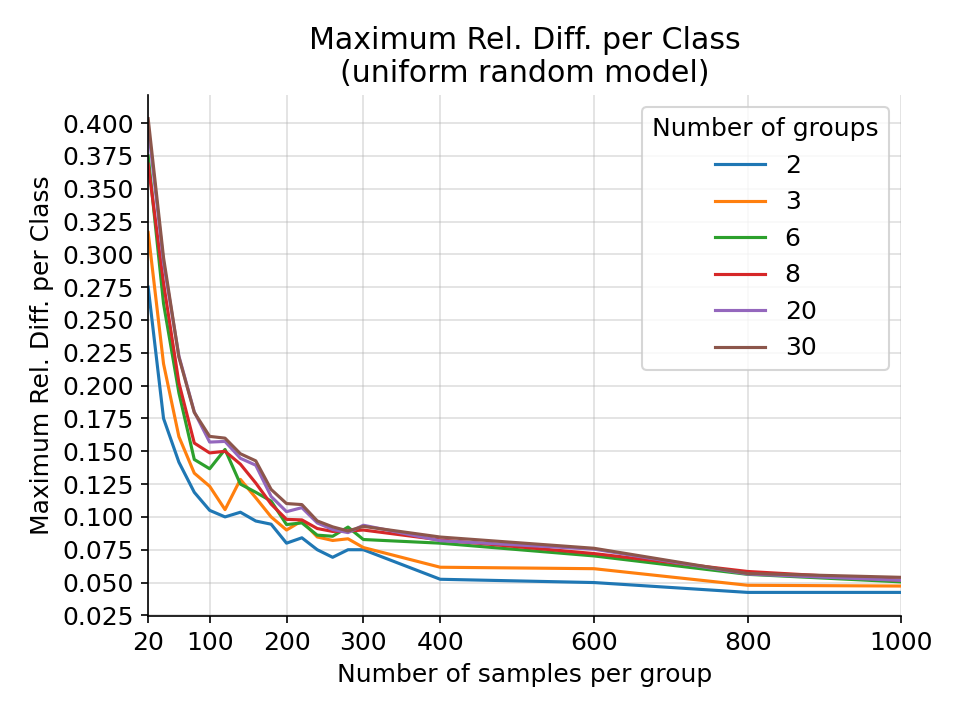
The maximum difference in relative difference per class for a random uniform categorical model from 1000 simulations.

Overview of tests and thresholds for arousal

Test	Threshold
Mean Value	0.075
Relative Difference Per Bin	0.225

Overview of tests and thresholds for dominance

Test	Threshold
Mean Value	0.075
Relative Difference Per Bin	0.225

Overview of tests and thresholds for valence

Test	Threshold
Mean Value	0.075
Relative Difference Per Bin	0.225

Overview of tests and thresholds for emotion

Test	Threshold
Relative Difference Per Class	0.225

Fairness Language

The models should not show a bias regarding the language of a speaker. As the perceived emotion is not independent of language and culture we don’t expect it to be without bias for all languages. In this test we focus on the main languages for which the model should be applied.

For each of the languages English, German, Italian, French, Spanish, and Chinese, 2000 random samples are selected. The prediction of the combined data is then compared against the prediction for each individual language.

The Mean Value over all samples should not change for any specific language compared to the combined database.

For the test Relative Difference Per Bin we follow Agarwal et al. [ADudikW19] and discretize the regression model outputs into 4 bins. The test checks that the number of samples per bin is comparable between the model prediction for one language and the model prediction for the combined database. We measure the difference of the number of samples in relative terms compared to the overall number of samples in the test set.

The test Relative Difference Per Class checks that the number of samples per class is comparable between the model prediction for one language and the model prediction for the combined database. We measure the difference of the number of samples in relative terms compared to the overall number of samples in the test set.

We base the thresholds on simulations with a random-categorical and a random-gaussian model for 6 fairness groups and at least 1000 samples per group, and increase them to accomodate for potential variations of the ground truth for different languages in the database. For the test Relative Difference Per Bin we require at least 67 predictions per bin in the combined dataset, or we skip that bin.

The maximum difference in mean difference for a random gaussian model from 1000 simulations.

The maximum difference in relative difference per bin for a random gaussian model from 1000 simulations.

The maximum difference in relative difference per class for a random uniform categorical model from 1000 simulations.

Overview of tests and thresholds for arousal

Test	Threshold
Mean Value	0.03
Relative Difference Per Bin	0.1

Overview of tests and thresholds for dominance

Test	Threshold
Mean Value	0.03
Relative Difference Per Bin	0.1

Overview of tests and thresholds for valence

Test	Threshold
Mean Value	0.03
Relative Difference Per Bin	0.1

Overview of tests and thresholds for emotion

Test	Threshold
Relative Difference Per Class	0.1

Fairness Linguistic Sentiment

The models should not show a bias regarding the language of a speaker. This also extends to the text sentiment that is contained in a sample. If the text content has an influence on the model predictions, it should have the same influence for each language.

We use the checklist-synth database, which contains synthetic speech of text with sentiment-labelled sentences or words generated from checklist. The text was generated from the English sentiment testing suite, and then translated into multiple languages. For each language, a publicly available speech-to-text model using both the libraries TTS and espnet was used to synthesize the audio samples corresponding to the text.

For each of the languages German, English, Spanish, French, Italian, Japanese, Portuguese, and Chinese up to 2000 random samples are selected per test set. The prediction of the combined data is then compared against the prediction for each individual language.

For this test we only want to measure the influence of text sentiment for different languages, and not general language biases, which are covered in the Fairness Language test. Therefore, we compare the shift in prediction when filtering the samples by a specific sentiment. We denote all samples with sentiment \(s\) and language \(l\) as \(X_{l, s}\), and all combined samples of language \(l\) as \(X_l\). We compute the difference between the shift in prediction for a certain sentiment and language and the average of the shifts in prediction for that sentiment for all languages \(l_i, 1 \leq i \leq L\)

\[\text{shift}(X_{l, s}) - \frac{1}{L}\sum_{i=1}^{L} \text{shift}(X_{l_i, s}).\]

The Mean Shift Difference Positive Sentiment, Mean Shift Difference Negative Sentiment, and Mean Shift Difference Neutral Sentiment tests compute the difference between the shift in mean value for one language and the average shift in mean value across all languages. They ensure that its absolute value is below a given threshold. The shift function of the tests is given by

\[\text{shift}_{\text{mean}}(X_{l, s}) = \text{mean}(\text{prediction}(X_{l, s})) - \text{mean}(\text{prediction}(X_l)).\]

For the tests Bin Proportion Shift Difference Positive Sentiment, Bin Proportion Shift Difference Negative Sentiment, and Bin Proportion Shift Difference Neutral Sentiment we follow Agarwal et al. [ADudikW19] and discretize the regression model outputs into 4 bins. The tests compute the difference between the shift in bin proportion for one language and the average shift in bin proportion across all languages. They ensure that its absolute value is below a given threshold. The shift function of the tests is given by

\[\begin{align*} \text{shift}_{b}(X_{l,s}) = & \frac{1}{| X_{l,s} |} | \{ y \; | \; y = b \; \text{and} \; y \in \text{prediction}_{\text{bin}}(X_{l, s}) \} | - \\ & \frac{1}{ | X_l |} | \{ y \; | \; y = b \; \text{and} \; y \in \text{prediction}_{\text{bin}}(X_{l}) \} |, \end{align*} \]

where \(b\) is the tested bin and \(\text{prediction}_{\text{bin}}\) is a function that applies the model to a given set of samples and assigns a bin label to each of the model outputs.

The tests Class Proportion Shift Difference Positive Sentiment, Class Proportion Shift Difference Negative Sentiment, and Class Proportion Shift Difference Neutral Sentiment compute the difference between the shift in class proportion for one language and the average shift in class proportion across all languages. They ensure that its absolute value is below a given threshold. The shift function of the tests is given by

\[\begin{align*} \text{shift}_{c}(X_{l,s}) = & \frac{1}{| X_{l,s} |} | \{ y \; | \; y = c \; \text{and} \; y \in \text{prediction}(X_{l, s}) \} | - \\ & \frac{1}{ | X_l |} | \{ y \; | \; y = c \; \text{and} \; y \in \text{prediction}(X_{l}) \} |, \end{align*} \]

where \(c\) is the tested class label.

We base the thresholds on simulations with a random-categorical and a random-gaussian model for 8 fairness groups and at least 1000 samples per group. For the Bin Proportion Shift Difference tests we require at least 67 predictions per bin in the combined dataset per sentiment, or we skip the bin for that sentiment.

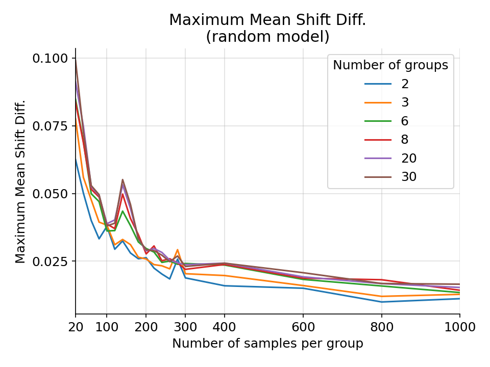
The maximum difference in mean shift difference for a random gaussian model from 1000 simulations.

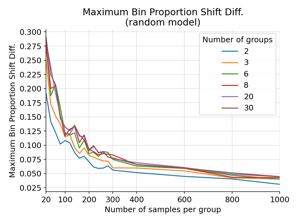
The maximum difference in bin proportion shift for a random gaussian model from 1000 simulations.

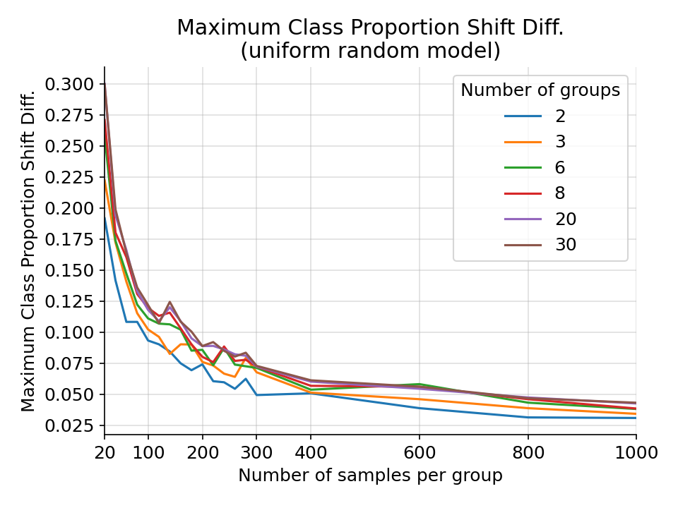
The maximum difference in class proportion shift for a random uniform categorical model from 1000 simulations.

Overview of tests and thresholds for arousal

Test	Threshold
Bin Proportion Shift Difference Negative Sentiment	0.075
Bin Proportion Shift Difference Neutral Sentiment	0.075
Bin Proportion Shift Difference Positive Sentiment	0.075
Mean Shift Difference Negative Sentiment	0.025
Mean Shift Difference Neutral Sentiment	0.025
Mean Shift Difference Positive Sentiment	0.025

Overview of tests and thresholds for dominance

Test	Threshold
Bin Proportion Shift Difference Negative Sentiment	0.075
Bin Proportion Shift Difference Neutral Sentiment	0.075
Bin Proportion Shift Difference Positive Sentiment	0.075
Mean Shift Difference Negative Sentiment	0.025
Mean Shift Difference Neutral Sentiment	0.025
Mean Shift Difference Positive Sentiment	0.025

Overview of tests and thresholds for valence

Test	Threshold
Bin Proportion Shift Difference Negative Sentiment	0.075
Bin Proportion Shift Difference Neutral Sentiment	0.075
Bin Proportion Shift Difference Positive Sentiment	0.075
Mean Shift Difference Negative Sentiment	0.025
Mean Shift Difference Neutral Sentiment	0.025
Mean Shift Difference Positive Sentiment	0.025

Overview of tests and thresholds for emotion

Test	Threshold
Class Proportion Shift Difference Negative Sentiment	0.075
Class Proportion Shift Difference Neutral Sentiment	0.075
Class Proportion Shift Difference Positive Sentiment	0.075

Fairness Pitch

The models should not show a bias regarding the average pitch of a speaker.

We only include speakers with more than 25 samples for this test. For each of these speakers, we compute the pitch of each sample. For pitch estimation we extract F0 framewise with praat and calculate a mean value for each segment, ignoring frames with a pitch value of 0 Hz. We exclude segments from the analysis that show a F0 below 50 Hz or above 350 Hz to avoid pitch estimation outlier to influence the tests. We then compute the average of all samples belonging to a speaker, and assign one of 3 pitch groups to that speaker. The low pitch group is assigned to speakers with an average pitch less than or equal to 145 Hz, the medium pitch group to speakers with an average pitch of more than 145 Hz but less than or equal to 190 Hz, and the high pitch group to speakers with an average pitch higher than 190 Hz.

We use two kinds of fairness criteria for this test. Firstly, we ensure that the performance for each pitch group is similar to the performance for the entire test set. Secondly, based on the principle of Equalized Odds [MMS+21] we ensure that we have similar values between each group and the entire test set for recall and precision for certain output classes.

The test thresholds are affected if the ground truth labels show a bias for a particular pitch group. To avoid this we first balance the test sets by selecting 1000 samples randomly from the pitch group with the fewest samples, and 1000 samples from the other pitch groups with similar truth values.

The Concordance Correlation Coeff High Pitch, Concordance Correlation Coeff Low Pitch, and Concordance Correlation Coeff Medium Pitch tests ensure that the difference in concordance correlation coefficient between the respective pitch group and the combined test set is below the given threshold.

For the tests Precision Per Bin High Pitch, Precision Per Bin Low Pitch, and Precision Per Bin Medium Pitch we discretize the regression model outputs into 4 bins and require that the difference in precision per bin between the respective pitch group and the combined test set is below the given threshold.

The Precision Per Class High Pitch, Precision Per Class Low Pitch, and Precision Per Class Medium Pitch tests ensure that the difference in precision per class between the respective pitch group and the combined test set is below the given threshold.

For the tests Recall Per Bin High Pitch, Recall Per Bin Low Pitch, and Recall Per Bin Medium Pitch we discretize the regression model outputs into 4 bins and require that the difference in recall per bin between the respective pitch group and the combined test set is below the given threshold.

The Recall Per Class High Pitch, Recall Per Class Low Pitch, and Recall Per Class Medium Pitch tests ensure that the difference in recall per class between the respective pitch group and the combined test set is below the given threshold.

The Unweighted Average Recall High Pitch, Unweighted Average Recall Low Pitch, and Unweighted Average Recall Medium Pitch tests ensure that the difference in unweighted average recall between the respective pitch group and the combined test set is below the given threshold.

We base the thresholds on simulations with a random-categorical and a random-gaussian model for 3 fairness groups and 1000 samples per group, and assume a sparse distribution of the ground truth for categories. For the Precision Per Bin and Recall Per Bin tests we require at least 67 samples per bin in the ground truth of the combined dataset, or we skip that bin.

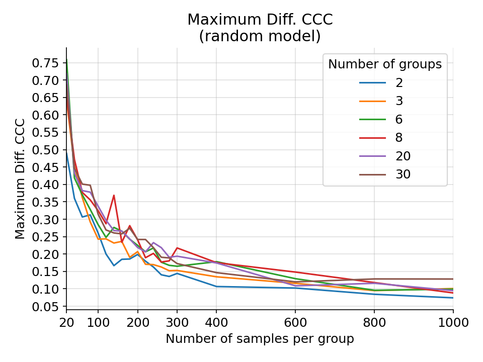
The maximum difference in CCC for a random gaussian model on a random gaussian ground truth from 1000 simulations.

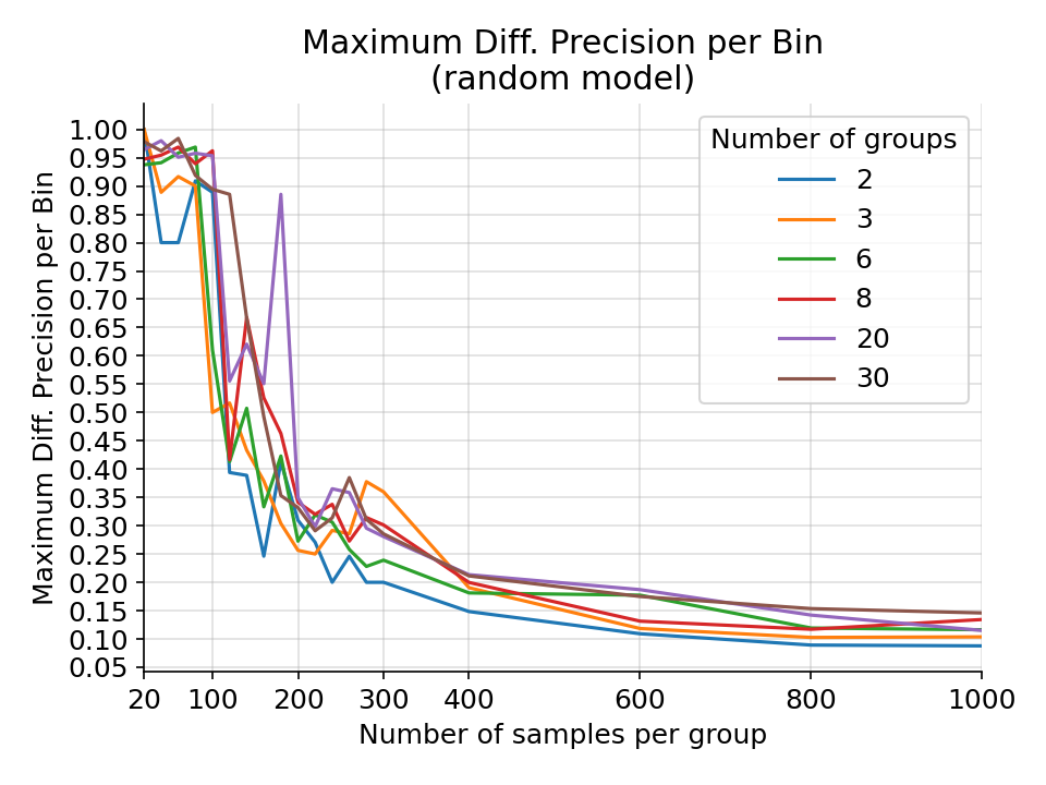
The maximum difference in precision per bin for a random gaussian model on a random gaussian ground truth from 1000 simulations.

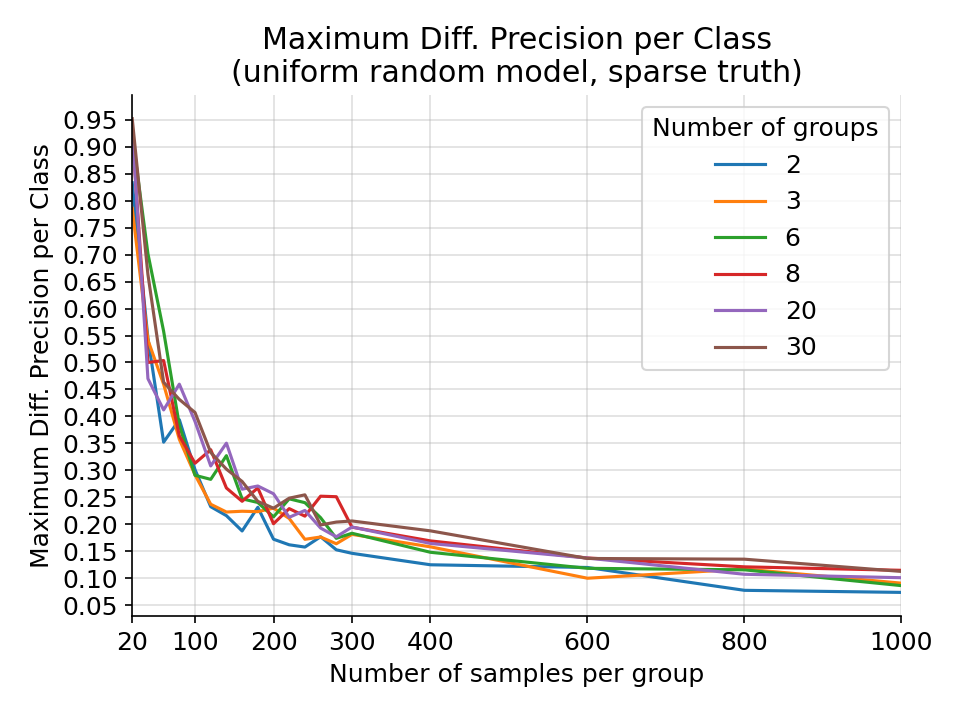
The maximum difference in precision per class for a random uniform categorical model on a random sparse categorical ground truth from 1000 simulations.

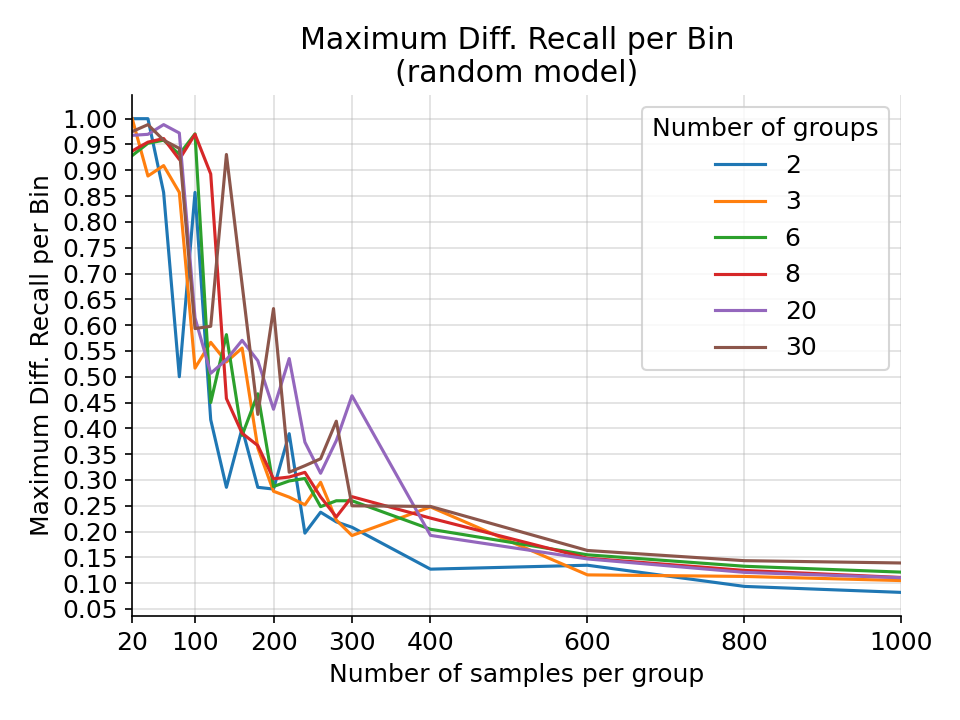
The maximum difference in recall per bin for a random gaussian model on a random gaussian ground truth from 1000 simulations.

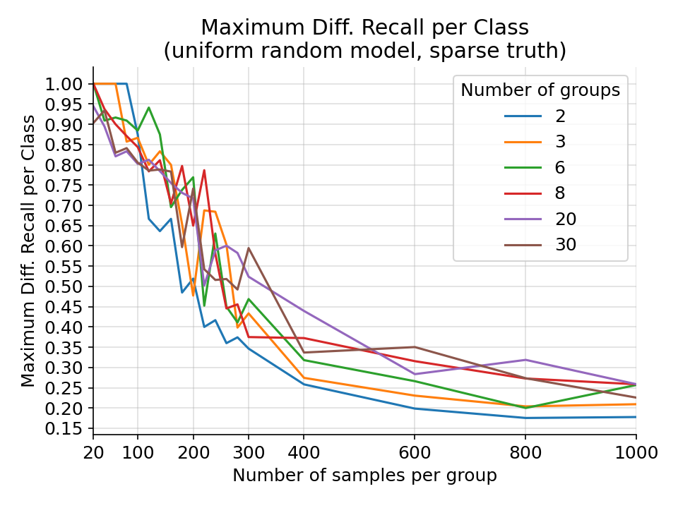
The maximum difference in precision per class for a random uniform categorical model on a random sparse categorical ground truth from 1000 simulations.

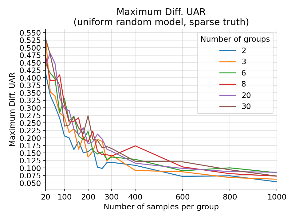
The maximum difference in UAR for a random uniform categorical model on a random sparse categorical ground truth from 1000 simulations.

Overview of tests and thresholds for arousal

Test	Threshold
Concordance Correlation Coeff High Pitch	0.1
Concordance Correlation Coeff Low Pitch	0.1
Concordance Correlation Coeff Medium Pitch	0.1
Precision Per Bin High Pitch	0.125
Precision Per Bin Low Pitch	0.125
Precision Per Bin Medium Pitch	0.125
Recall Per Bin High Pitch	0.125
Recall Per Bin Low Pitch	0.125
Recall Per Bin Medium Pitch	0.125

Overview of tests and thresholds for dominance

Test	Threshold
Concordance Correlation Coeff High Pitch	0.1
Concordance Correlation Coeff Low Pitch	0.1
Concordance Correlation Coeff Medium Pitch	0.1
Precision Per Bin High Pitch	0.125
Precision Per Bin Low Pitch	0.125
Precision Per Bin Medium Pitch	0.125
Recall Per Bin High Pitch	0.125
Recall Per Bin Low Pitch	0.125
Recall Per Bin Medium Pitch	0.125

Overview of tests and thresholds for valence

Test	Threshold
Concordance Correlation Coeff High Pitch	0.1
Concordance Correlation Coeff Low Pitch	0.1
Concordance Correlation Coeff Medium Pitch	0.1
Precision Per Bin High Pitch	0.125
Precision Per Bin Low Pitch	0.125
Precision Per Bin Medium Pitch	0.125
Recall Per Bin High Pitch	0.125
Recall Per Bin Low Pitch	0.125
Recall Per Bin Medium Pitch	0.125

Overview of tests and thresholds for emotion

Test	Threshold
Precision Per Class High Pitch	0.1
Precision Per Class Low Pitch	0.1
Precision Per Class Medium Pitch	0.1
Recall Per Class High Pitch	0.225
Recall Per Class Low Pitch	0.225
Recall Per Class Medium Pitch	0.225
Unweighted Average Recall High Pitch	0.075
Unweighted Average Recall Low Pitch	0.075
Unweighted Average Recall Medium Pitch	0.075

Fairness Sex

The models should not show a bias regarding the sex of a speaker.

We use two kinds of fairness criteria for this test. Firstly, we ensure that the performance for each sex is similar to the performance for the entire test set. Secondly, based on the principle of Equalized Odds [MMS+21] we ensure that we have similar values between each sex and the entire test set for recall and precision for certain output classes.

The test thresholds are affected if the ground truth labels show a bias for a particular sex. To avoid this we first balance the test sets by selecting 1000 samples randomly from the sex group with the fewest samples, and 1000 samples from the other sex group with similar truth values.

The Concordance Correlation Coeff Female and Concordance Correlation Coeff Male tests ensure that the difference in concordance correlation coefficient between the respective sex and the combined test set is below the given threshold.

For the tests Precision Per Bin Female and Precision Per Bin Male we discretize the regression model outputs into 4 bins and require that the difference in precision per bin between the respective sex and the combined test set is below the given threshold.

The Precision Per Class Female and Precision Per Class Male tests ensure that the difference in precision per class between the respective sex and the combined test set is below the given threshold.

For the tests Recall Per Bin Female and Recall Per Bin Male we discretize the regression model outputs into 4 bins and require that the difference in recall per bin between the respective sex and the combined test set is below the given threshold.

The Recall Per Class Female and Recall Per Class Male tests ensure that the difference in recall per class between the respective sex and the combined test set is below the given threshold.

The Unweighted Average Recall Female and Unweighted Average Recall Male tests ensure that the difference in unweighted average recall between the respective sex and the combined test set is below the given threshold.

We base the thresholds on simulations with a random-categorical and a random-gaussian model for 2 fairness groups and 1000 samples per group, and assume a sparse distribution of the ground truth for categories. For the Precision Per Bin and Recall Per Bin tests we require at least 67 samples per bin in the ground truth of the combined dataset, or we skip that bin.

The maximum difference in CCC for a random gaussian model on a random gaussian ground truth from 1000 simulations.

The maximum difference in precision per bin for a random gaussian model on a random gaussian ground truth from 1000 simulations.

The maximum difference in precision per class for a random uniform categorical model on a random sparse categorical ground truth from 1000 simulations.

The maximum difference in recall per bin for a random gaussian model on a random gaussian ground truth from 1000 simulations.

The maximum difference in recall per class for a random uniform categorical model on a random sparse categorical ground truth from 1000 simulations.

The maximum difference in UAR for a random uniform categorical model on a random sparse categorical ground truth from 1000 simulations.

Overview of tests and thresholds for arousal

Test	Threshold
Concordance Correlation Coeff Female	0.075
Concordance Correlation Coeff Male	0.075
Precision Per Bin Female	0.1
Precision Per Bin Male	0.1
Recall Per Bin Female	0.1
Recall Per Bin Male	0.1

Overview of tests and thresholds for dominance

Test	Threshold
Concordance Correlation Coeff Female	0.075
Concordance Correlation Coeff Male	0.075
Precision Per Bin Female	0.1
Precision Per Bin Male	0.1
Recall Per Bin Female	0.1
Recall Per Bin Male	0.1

Overview of tests and thresholds for valence

Test	Threshold
Concordance Correlation Coeff Female	0.075
Concordance Correlation Coeff Male	0.075
Precision Per Bin Female	0.1
Precision Per Bin Male	0.1
Recall Per Bin Female	0.1
Recall Per Bin Male	0.1

Overview of tests and thresholds for emotion

Test	Threshold
Precision Per Class Female	0.075
Precision Per Class Male	0.075
Recall Per Class Female	0.175
Recall Per Class Male	0.175
Unweighted Average Recall Female	0.075
Unweighted Average Recall Male	0.075

Robustness Background Noise

We show in the Robustness Small Changes test, that our emotion models’ predictions might change when adding white noise to the input signal. Similar results are known from the speech emotion recognition literature. Jaiswal and Provost [JP21] have shown that adding environmental noise like rain or coughing, leads to a drop of performance of around 50% for a signal-to-noise ratio of 20 dB.

The purpose of this test is to investigate how the model performance is influenced by different added noises at lower signal-to-noise ratios as used in the Robustness Small Changes test. As background noises we use the following:

• Babble Noise: 4 to 7 speech samples from the speech table of the musan database [SGCP15] are mixed and added with an SNR of 20 dB

• Coughing: one single cough from our internal cough-speech-sneeze database (based on [APC+17]) is added to each sample at a random position with an SNR of 10 dB

• Environmental Noise: a noise sample from the noise table of the musan database is added with an SNR of 20 dB. The noise table includes technical noises, such as DTMF tones, dialtones, fax machine noises, and more, as well as ambient sounds, such as car idling, thunder, wind, footsteps, paper rustling, rain, animal noises

• Music: a music sample from the music table of the musan database is added with an SNR of 20 dB. The music table includes Western art music (e.g. Baroque, Romantic, Classical) and popular genres (e.g. jazz, bluegrass, hiphop)

• Sneezing: one single sneeze from the cough-speech-sneeze database is added to each sample at a random position with an SNR of 10 dB

• White Noise: white noise is added with an SNR of 20 dB

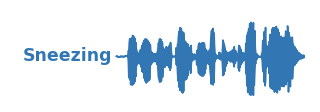
The Change CCC Babble Noise, Change CCC Coughing, Change CCC Environmental Noise, Change CCC Music, Change CCC Sneezing, and Change CCC White Noise tests ensure that the Concordance Correlation Coefficient (CCC) does not decrease too much when adding the given background noise.

The Change UAR Babble Noise, Change UAR Coughing, Change UAR Environmental Noise, Change UAR Music, Change UAR Sneezing, and Change UAR White Noise tests ensure that the Unweighted Average Recall (UAR) does not decrease too much when adding the given background noise.

The Percentage Unchanged Predictions Babble Noise, Percentage Unchanged Predictions Coughing, Percentage Unchanged Predictions Environmental Noise, Percentage Unchanged Predictions Music, Percentage Unchanged Predictions Sneezing, Percentage Unchanged Predictions White Noise tests check that the percentage of samples with unchanged predictions is high enough when adding the given background noise. We use the same definitions as in the Robustness Small Changes to compute this percentage.

Overview of tests and thresholds for arousal

Test	Threshold
Change Ccc Babble Noise	-0.05
Change Ccc Coughing	-0.05
Change Ccc Environmental Noise	-0.05
Change Ccc Music	-0.05
Change Ccc Sneezing	-0.05
Change Ccc White Noise	-0.05
Percentage Unchanged Predictions Babble Noise	0.9
Percentage Unchanged Predictions Coughing	0.9
Percentage Unchanged Predictions Environmental Noise	0.9
Percentage Unchanged Predictions Music	0.9
Percentage Unchanged Predictions Sneezing	0.9
Percentage Unchanged Predictions White Noise	0.9

Overview of tests and thresholds for dominance

Test	Threshold
Change Ccc Babble Noise	-0.05
Change Ccc Coughing	-0.05
Change Ccc Environmental Noise	-0.05
Change Ccc Music	-0.05
Change Ccc Sneezing	-0.05
Change Ccc White Noise	-0.05
Percentage Unchanged Predictions Babble Noise	0.9
Percentage Unchanged Predictions Coughing	0.9
Percentage Unchanged Predictions Environmental Noise	0.9
Percentage Unchanged Predictions Music	0.9
Percentage Unchanged Predictions Sneezing	0.9
Percentage Unchanged Predictions White Noise	0.9

Overview of tests and thresholds for valence

Test	Threshold
Change Ccc Babble Noise	-0.05
Change Ccc Coughing	-0.05
Change Ccc Environmental Noise	-0.05
Change Ccc Music	-0.05
Change Ccc Sneezing	-0.05
Change Ccc White Noise	-0.05
Percentage Unchanged Predictions Babble Noise	0.9
Percentage Unchanged Predictions Coughing	0.9
Percentage Unchanged Predictions Environmental Noise	0.9
Percentage Unchanged Predictions Music	0.9
Percentage Unchanged Predictions Sneezing	0.9
Percentage Unchanged Predictions White Noise	0.9

Overview of tests and thresholds for emotion

Test	Threshold
Change Uar Babble Noise	-0.05
Change Uar Coughing	-0.05
Change Uar Environmental Noise	-0.05
Change Uar Music	-0.05
Change Uar Sneezing	-0.05
Change Uar White Noise	-0.05
Percentage Unchanged Predictions Babble Noise	0.9
Percentage Unchanged Predictions Coughing	0.9
Percentage Unchanged Predictions Environmental Noise	0.9
Percentage Unchanged Predictions Music	0.9
Percentage Unchanged Predictions Sneezing	0.9
Percentage Unchanged Predictions White Noise	0.9

Robustness Low Quality Phone

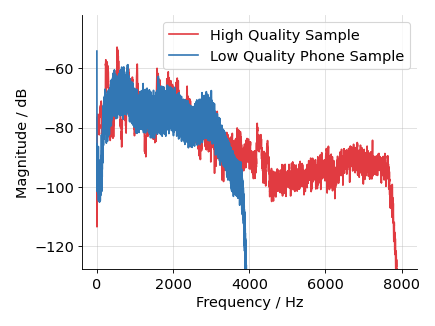
The models should be robust to a low quality phone recording condition. Low quality phone recordings usually have stronger compression, and coding artifacts. In addition, they may show low pass behavior as indicated by the following plot showing the magnitude spectrum for one low quality phone sample from switchboard-1, and a high quality headphone recording sample from emovo.

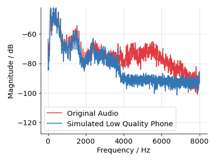
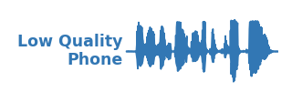
We mimic this behavior by applying a dynamic range compressor with a threshold of -20 dB, a ratio of 0.8, attack time of 0.01 s, and a release time of 0.02 s to the incoming high quality signal. The outgoing signal is then encoded by the lossy Adaptive Multi-Rate (AMR) codec with a bit rate of 7400 using its narrow band version which involves a downsampling to 8000 Hz. The signal is afterwards upsampled to 16000 Hz, peak normalized, and we add high pass filtered pink noise with a gain of -25 dB. The high pass employs a cutoff frequency of 3000 Hz and an order of 2. When applying the filters we ensure that the overall signal level stays the same if possible without clipping.

We use the same definitions as in Robustness Small Changes to compute the difference \(\delta\) in prediction.

The Change CCC Low Quality Phone test ensures that the Concordance Correlation Coefficient (CCC) does not decrease further than by the given threshold when applying the low quality phone filter.

The Change UAR Low Quality Phone tests ensure that the Unweighted Average Recall (UAR) does not decrease too much when applying the low quality phone filter.

The Percentage Unchanged Predictions Low Quality Phone tests check that the percentage of samples with unchanged predictions is high enough when applying the low quality phone filter. We use the same definitions as in the Robustness Small Changes to compute this percentage.

Overview of tests and thresholds for arousal

Test	Threshold
Change Ccc Low Quality Phone	-0.05
Percentage Unchanged Predictions Low Quality Phone	0.5

Overview of tests and thresholds for dominance

Test	Threshold
Change Ccc Low Quality Phone	-0.05
Percentage Unchanged Predictions Low Quality Phone	0.5

Overview of tests and thresholds for valence

Test	Threshold
Change Ccc Low Quality Phone	-0.05
Percentage Unchanged Predictions Low Quality Phone	0.5

Overview of tests and thresholds for emotion

Test	Threshold
Change Uar Low Quality Phone	-0.05
Percentage Unchanged Predictions Low Quality Phone	0.5

Robustness Recording Condition

The models should not change their output when using a different microphone or a different microphone position to record the same audio. To test this, we use databases that have simultaneous recordings of the same audio with different microphones and with different positions.

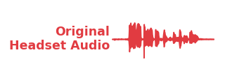
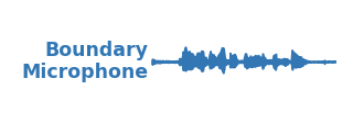
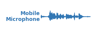
The Percentage Unchanged Predictions Recording Condition test compares the prediction on the audio in one recording condition to the same audio in another recording condition, and checks that the percentage of unchanged predictions is high enough. We use the same definitions as in the Robustness Small Changes to compute this percentage.

Overview of tests and thresholds for arousal

Test	Threshold
Percentage Unchanged Predictions Recording Condition	0.8

Overview of tests and thresholds for dominance

Test	Threshold
Percentage Unchanged Predictions Recording Condition	0.8

Overview of tests and thresholds for valence

Test	Threshold
Percentage Unchanged Predictions Recording Condition	0.8

Overview of tests and thresholds for emotion

Test	Threshold
Percentage Unchanged Predictions Recording Condition	0.8

Robustness Simulated Recording Condition

As described in the Robustness Recording Condition test, the models should give the same or at least a similar output for the same audio but recorded in different conditions. To expand on the Robustness Recording Condition test we simulate different recording conditions in this test.

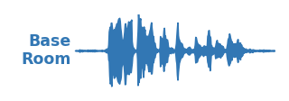
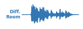
We augment clean speech samples with impulse responses corresponding to different audio locations from the mardy database [WGH+06] as well as impulse responses corresponding to different rooms from the air database [JSV09]. For the position test we use the impulse response in the center position at 1 meter distance as the base (or reference) position to compare all other positions to. For the room test we use the impulse response of a recording booth and compare to impulse responses of other rooms recorded at similar distances as the reference impulse response.

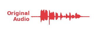
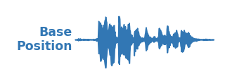
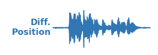
The Percentage Unchanged Predictions Simulated Position test compares the prediction on the audio with a simulated base position to that of the same audio with a different simulated position, and checks that the percentage of samples with unchanged predictions is high enough. We use the same definitions as in the Robustness Small Changes to compute this percentage.

The Percentage Unchanged Predictions Simulated Room test compares the prediction on the audio with a simulated base room to that of the same audio with a different simulated room, and checks that the percentage of samples with unchanged predictions is high enough. We use the same definitions as in the Robustness Small Changes to compute this percentage.

Overview of tests and thresholds for arousal

Test	Threshold
Percentage Unchanged Predictions Simulated Position	0.8
Percentage Unchanged Predictions Simulated Room	0.8

Overview of tests and thresholds for dominance

Test	Threshold
Percentage Unchanged Predictions Simulated Position	0.8
Percentage Unchanged Predictions Simulated Room	0.8

Overview of tests and thresholds for valence

Test	Threshold
Percentage Unchanged Predictions Simulated Position	0.8
Percentage Unchanged Predictions Simulated Room	0.8

Overview of tests and thresholds for emotion

Test	Threshold
Percentage Unchanged Predictions Simulated Position	0.8
Percentage Unchanged Predictions Simulated Room	0.8

Robustness Small Changes

The models should not change their output if we apply very small changes to the input signals. To test this we apply small changes to the input signal and compare the predictions. For regression, we calculate the difference \(\delta_\text{reg}\) in prediction

\[\delta_\text{reg}(\text{segment}_s) = \| \text{prediction}_\text{reg}(\text{segment}_s) - \text{prediction}_\text{reg}(\text{augment}(\text{segment}_s)) \|\]

for each segment \(\text{segment}_s\), with \(\text{prediction}_\text{reg}(\cdot) \in [0, 1]\). The percentage of unchanged predictions for regression is then given by the percentage of all segments \(S\) with \(\delta_\text{reg} < 0.05\):

\[\text{percentage\_unchanged}_\text{reg} = \frac{ | \{\text{segment}_s \; | \; \delta_\text{reg}(\text{segment}_s) < 0.05 \; \text{and} \; 1 \leq s \leq S\} | }{ | \{\text{segment}_s \; | \; 1 \leq s \leq S\} | }\]

For classification the difference \(\delta_\text{cls}\) in prediction is given by

\[\delta_\text{cls}(\text{segment}_s) = \| \text{prediction}_\text{cls}(\text{segment}_s) - \text{prediction}_\text{cls}(\text{augment}(\text{segment}_s)) \|_2\]

for each segment \(\text{segment}_s\), with \(\text{prediction}_\text{cls}(\cdot) \in \{\mathbf{e}^{(i)} \; | \; 1 \leq i \leq C\}\), where \(\mathbf{e}^{(i)}\) is a one-hot vector corresponding to one of the \(C\) classes. The percentage of unchanged predictions for classification is then given by the percentage of all segments \(S\) with \(\delta_\text{cls} = 0\):

\[\text{percentage\_unchanged}_\text{cls} = \frac{ | \{\text{segment}_s \; | \; \delta_\text{cls}(\text{segment}_s) = 0 \; \text{and} \; 1 \leq s \leq S\} | }{ | \{\text{segment}_s \; | \; 1 \leq s \leq S\} | }\]

All the changes we apply here, were optimized by listening to one example augmented audio file and adjusting the settings so that a user perceives the changes as subtle.

The Percentage Unchanged Predictions Additive Tone test adds a sinusoid with a frequency randomly selected between 5000 Hz and 7000 Hz, with a peak based signal-to-noise ratio randomly selected from 40 dB, 45 dB, 50 dB and checks that the percentage of unchanged predictions is above the given threshold.

The Percentage Unchanged Predictions Append Zeros test adds samples containing zeros at the end of the input signal and checks that the percentage of unchanged predictions is above the given threshold. The number of samples is randomly selected from 100, 500, 1000.

The Percentage Unchanged Predictions Clip test clips a given percentage of the input signal and checks that the percentage of unchanged predictions is above the given threshold. The clipping percentage is randomly selected from 0.1%, 0.2%, 0.3%

The Percentage Unchanged Predictions Crop Beginning test removes samples from the beginning of an input signal and checks that the percentage of unchanged predictions is above the given threshold. The number of samples is randomly selected from 100, 500, 1000.

The Percentage Unchanged Predictions Crop End test removes samples from the end of an input signal and checks that the percentage of unchanged predictions is above the given threshold. The number of samples is randomly selected from 100, 500, 1000.

The Percentage Unchanged Predictions Gain test changes the gain of an input signal by a value randomly selected from -2 dB, -1 dB, 1 dB, 2 dB and checks that the percentage of unchanged predictions is above the given threshold.

The Percentage Unchanged Predictions Highpass Filter test applies a high pass Butterworth filter of order 1 to the input signal with a cutoff frequency randomly selected from 50 Hz, 100 Hz, 150 Hz and checks that the percentage of unchanged predictions is above the given threshold.

The Percentage Unchanged Predictions Lowpass Filter test applies a low pass Butterworth filter of order 1 to the input signal with a cutoff frequency randomly selected from 7500 Hz, 7000 Hz, 6500 Hz and checks that the percentage of unchanged predictions is above the given threshold.

The Percentage Unchanged Predictions Prepend Zeros test adds samples containing zeros at the beginning of the input signal and checks that the percentage of unchanged predictions is above the given threshold. The number of samples is randomly selected from 100, 500, 1000.

The Percentage Unchanged Predictions White Noise test adds Gaussian distributed white noise to the input signal with a root mean square based signal-to-noise ratio randomly selected from 35 dB, 40 dB, 45 dB and checks that the percentage of unchanged predictions is above the given threshold.

Overview of tests and thresholds for arousal

Test	Threshold
Percentage Unchanged Predictions Additive Tone	0.95
Percentage Unchanged Predictions Append Zeros	0.95
Percentage Unchanged Predictions Clip	0.95
Percentage Unchanged Predictions Crop Beginning	0.95
Percentage Unchanged Predictions Crop End	0.95
Percentage Unchanged Predictions Gain	0.95
Percentage Unchanged Predictions Highpass Filter	0.95
Percentage Unchanged Predictions Lowpass Filter	0.95
Percentage Unchanged Predictions Prepend Zeros	0.95
Percentage Unchanged Predictions White Noise	0.95

Overview of tests and thresholds for dominance

Test	Threshold
Percentage Unchanged Predictions Additive Tone	0.95
Percentage Unchanged Predictions Append Zeros	0.95
Percentage Unchanged Predictions Clip	0.95
Percentage Unchanged Predictions Crop Beginning	0.95
Percentage Unchanged Predictions Crop End	0.95
Percentage Unchanged Predictions Gain	0.95
Percentage Unchanged Predictions Highpass Filter	0.95
Percentage Unchanged Predictions Lowpass Filter	0.95
Percentage Unchanged Predictions Prepend Zeros	0.95
Percentage Unchanged Predictions White Noise	0.95

Overview of tests and thresholds for valence

Test	Threshold
Percentage Unchanged Predictions Additive Tone	0.95
Percentage Unchanged Predictions Append Zeros	0.95
Percentage Unchanged Predictions Clip	0.95
Percentage Unchanged Predictions Crop Beginning	0.95
Percentage Unchanged Predictions Crop End	0.95
Percentage Unchanged Predictions Gain	0.95
Percentage Unchanged Predictions Highpass Filter	0.95
Percentage Unchanged Predictions Lowpass Filter	0.95
Percentage Unchanged Predictions Prepend Zeros	0.95
Percentage Unchanged Predictions White Noise	0.95

Overview of tests and thresholds for emotion

Test	Threshold
Percentage Unchanged Predictions Additive Tone	0.95
Percentage Unchanged Predictions Append Zeros	0.95
Percentage Unchanged Predictions Clip	0.95
Percentage Unchanged Predictions Crop Beginning	0.95
Percentage Unchanged Predictions Crop End	0.95
Percentage Unchanged Predictions Gain	0.95
Percentage Unchanged Predictions Highpass Filter	0.95
Percentage Unchanged Predictions Lowpass Filter	0.95
Percentage Unchanged Predictions Prepend Zeros	0.95
Percentage Unchanged Predictions White Noise	0.95

Robustness Spectral Tilt

The models should be robust against boosting low or high frequencies in the spectrum. We simulate such spectral tilts by attenuating or emphasizing the signal linearly. This is achieved by convolving the signal with appropriate filters as shown in the figure below.

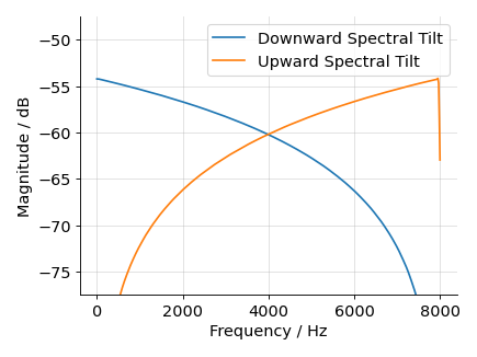
When applying the filters we ensure that the overall signal level stays the same if possible without clipping.

The Change CCC Downward Tilt and Change CCC Upward Tilt tests ensure that the Concordance Correlation Coefficient (CCC) does not decrease too much when applying the downward or upward spectral tilt filter.

The Change UAR Downward Tilt and Change UAR Upward Tilt tests ensure that the Unweighted Average Recall (UAR) does not decrease too much when applying the downward or upward spectral tilt filter.

The Percentage Unchanged Predictions Downward Tilt and Percentage Unchanged Predictions Upward Tilt tests check that the percentage of samples with unchanged predictions is high enough when applying the downward or upward spectral tilt filter. We use the same definitions as in the Robustness Small Changes to compute this percentage.

Overview of tests and thresholds for arousal

Test	Threshold
Change Ccc Downward Tilt	-0.05
Change Ccc Upward Tilt	-0.05
Percentage Unchanged Predictions Downward Tilt	0.8
Percentage Unchanged Predictions Upward Tilt	0.8

Overview of tests and thresholds for dominance

Test	Threshold
Change Ccc Downward Tilt	-0.05
Change Ccc Upward Tilt	-0.05
Percentage Unchanged Predictions Downward Tilt	0.8
Percentage Unchanged Predictions Upward Tilt	0.8

Overview of tests and thresholds for valence

Test	Threshold
Change Ccc Downward Tilt	-0.05
Change Ccc Upward Tilt	-0.05
Percentage Unchanged Predictions Downward Tilt	0.8
Percentage Unchanged Predictions Upward Tilt	0.8

Overview of tests and thresholds for emotion

Test	Threshold
Change Uar Downward Tilt	-0.02
Change Uar Upward Tilt	-0.02
Percentage Unchanged Predictions Downward Tilt	0.8
Percentage Unchanged Predictions Upward Tilt	0.8